Losing your RAG

Variations of the Red-Amber-Green "RAG" performance rating system are used extensively. 

A common version is really a two rating (Red-Green) system i.e. where all performance is marked as either pass or fail. When over-used on a table of numbers (not least  with the common practice of colouring whole cells), this can produce a confusing and garish grid. 

A proper three-grade RAG system, including the central Amber, allows more sophisticated ratings to be made. But the Amber rating can be used in two very different ways:

• Fail but only just
• Pass but close to fail

Either way, including Amber in the pattern of fully coloured cells just adds further to the over-whelming blast of colour that assaults the reader's brain.

So why, so often,  do we end up with these types of reports and dashboards? 

The whole cell colour aspect  is probably mainly down to ease of production. It is much easier to produce this in say, Excel, than to use less over-whelming devices. 

The extensive use of Green is more curious. It probably indicates a service area where performance has regularly been below target and the people concerned are feeling a bit battered.  Lots of Red is demoralising so every opportunity is taken to proclaim the Green. The same motivation will probably lead to adopting the Amber "fail but only just" option. It removes more Red and it gives a feeling of "nearly there".

But before jumping into producing another one of these grids, the analyst should consider what the report or dashboard is actually trying to communicate. In the end, the main purpose has to be to highlight to managers when they need to make a decision or initiate action. 

This being so, what is the purpose of the Green? There are lots of months where the target was achieved. So what? What action will we take? Apart, possibly, from a momentary congratulation  - none. The Green is where we want to be. Colouring it in may give a sense of assurance, but it does not trigger any management action.

The Red rating is more obvious: we have not achieved the target and we need to do something.

What about Amber? A "fail but only just" statement is still a fail. We still need to do something. What we really need to know is where we met the target (Green) but only just. This is a situation where things may deteriorate and become Red. We may need to take action soon, or be pro-active and take action now, so we need to highlight this.

These considerations suggest that what would be best is a "RA" rating i.e. Red (fail) and Amber (pass but only just) system. Leave everything else un-highlighted on the grounds that there is no need to draw attention to it.

An example could look something like

where Red indicates that we missed the target and Amber indicates that we achieved the target but it was so close to the borderline that we may need to act, or at least keep a close eye on it.

This type of Red-Amber rating system can be developed further to make the Amber look more like a faint Red i.e to use a monochrome (Red-red) system in which tone conveys the meaning. Using this approach, together with some further adjustments to contrast, gives the following alternative:

This illustration uses exactly the same data as the grid above but is set out in a very different way. The idea is to adjust the contrast so that important information stands out and less important information melts into the background. 

Attention is drawn to the latest position rather than to the history of previous results. Indicator 4,  which missed the target is clearly highlighted by the Red marker. Two other indicators (5 and 7), which  only just hit the target, are also highlighted, but in a lighter tone.

The compact visual summary of the last six results then provides additional detail. Indicator 5 has generally been ok so there is probably no need to over-react. Indicator 7 has a history of missing the target. We should continue to monitor it closely.

In conclusion, for dashboards and reports, it may often make sense to abandon the customary RAG systems in favour of a Red-Amber (RA) or Red-red (Rr) as described here.

Finally, another practical reason to abandon the RAG is to help the 10% of males, and 1% of females,  who are colour blind.


References

3 Problems With Traditional KPI Traffic Lights by Stacey Barr. 20/05/2014

(link)

Dashboard Design for Real-Time Situation Awareness by Stephen Few. 2007 (link)


Excel: creating a 'Last Ten Results' indicator panel without using VBA by Edgar Bolton. B I Dashboard Design. 31/01/2016  (link)

Why month-based views are unsuitable for data which exhibits weekly patterns

One of the most commonly encountered formats for presenting data is a table of monthly totals,  often accompanied by a graph.

One reason for the extensive use of this approach is that it is very familiar and is practically self-perpetuating. It almost suggests itself.

Another reason is that it is a relatively easy calculation to produce month based counts using commonly available tools such as Excel, Access, SQL. Producing weekly aggregate numbers from raw data is a slightly higher level of difficulty. Similarly, producing a graph in Excel from a table of monthly totals is almost effortless. Producing an SPC (Statistical Process Control) type run chart is a little less easy.

A monthly review makes perfectly good sense. It is a reasonable time interval against which to assess a progress. Much less than a month and we risk over-reacting to short term fluctuations; much more than a month and we may not give ourselves enough time to act.

Where things can go wrong is where a good time interval for review gets confused with a good time interval for analysis.

Unfortunately there are many situations where a month-by-month view masks, rather than highlights, the real patterns in the data. People presented with a month by month graph in which the numbers go up and down will feel that they are seeing the real changes in activity. They may be reassured if the numbers go the 'right' way and panic if the numbers seem to go in the opposite direction.

The following illustration shows a series of monthly counts of events:

The monthly totals time series shows numbers going up and down suggesting a pattern of changing activity. 

Most readers will quickly spot that the pattern in the graph is nothing more than a representation of the number of days in each month. It has been built up from exactly 10 events each day throughout the entire period being studied. Nothing is changing at all.

The appearance of changing activity has been exaggerated by the default behaviour of Excel in truncating the vertical axis when creating graphs.

A way of compensating for this is to divide the total number of events in the month by the number of days in the month i.e. to calculate a daily rate. This is added on the illustration above. It shows that the monthly pattern of activity is actually static. 

For analysis, the rule should be that where the period being studied is divided up into unequal time periods (such as months), it is better to use a rate than to use a simple period total. It is surprising how often this simple rule is not followed.

In many situations, this compensating technique (translation into rates) may not be sufficient. The next illustration shows a series of monthly counts of events. The daily rate has been calculated. The rate goes up and down, suggesting change:

However, here again, the impression of a changing levels of activity is an illusion. 

The underlying pattern of activity is really static. It is a constant 28 events a week throughout the study period. For the purposes of illustration, the weekly pattern synthesised for the illustration has been strongly polarised (All Mondays have 7 events, Tuesdays 6 events, etc down to Sundays with 1 event). 

The spurious pattern in the illustration results from the interplay between the consistent but uneven distribution within each week in combination with the disposition of weeks across month end boundaries.

Another regularly used 'compensatory' technique is to show a monthly total alongside the equivalent month from the previous year:

Surely this approach is valid as, with the exception of some Februaries, we are comparing the activity in exactly equivalent time periods, side by side?

Unfortunately, again, the appearance of changing activity is an illusion. The graph is derived from exactly the same static pattern of 28 events per week as was used in the previous illustration.

If this is what static data looks like through this framework, imagine how hard it would be to make sense of any real patterns of change.

In areas where there are strong weekly patterns, such as healthcare, viewing data through the distortion of a monthly framework makes it very difficult to see what is really going on.

So while monthly views work well for appropriate uses, such as showing cumulative income year-to-date, they will often be a poor choice for displaying and understanding patterns of event activity. 

Unlike the month, the week is a more 'natural' time period which aligns well with patterns of behaviour. It is worth the extra effort of aggregating event data by week and looking at it in weekly run charts. The SPC method can be used to assess whether the variation seen reflects any real changes.

At the very least, a preliminary analysis will be needed to assess the strength of weekly patterns in the data before a decision can be made on how much 'noise' this is likely to create in a monthly time series .

Another technique used in reports and dashboards is to divide monthly totals of events by the number of 'working days' in a month. This can go some way towards making comparisons better. But it still does not compensate fully for a strong weekly pattern. 

Also, it would be necessary to review each measure being reported on and assign an individual number of working days to it. This can vary from measure to measure. Some events would be expected to occur on weekends and bank holidays. Some services may operate for less than five days a week. It cannot be assumed that using the number of 'working days' worked by the analyst in the month is the correct denominator in every, or even any, case.

Excel: adding interactive drill down to a 'Last Ten Results' indicator panel

A previous article outlined a simple method for creating a 'Last Ten Results' indicator panel in Excel (see link). This supplement shows how to add interactive drill down functionality (Excel skill level: advanced)

Another previous article had shown how to use Excel comments boxes dynamically to provide drill down details (see link). This method can be adapted to work with the last ten results indicator panel. There are a few technical challenges.

Reversing a linking formula
The cells coloured green,  red and grey in the indicator panel read values from a separate data area. The way the data is structured (in this example) the drill-down needs to read from three adjacent rows in the data area, e.g. cells AF10, AF11, AF12.  This is trickier than it first seems. 

Some VBA code which can do this set out below. It is triggered by the Worksheet Selection Change event i.e.the code is run each time a different area on the worksheet is selected. So the code is run when any of the coloured bars are clicked on, displaying the appropriate details for the cell It is run again when any non bar cell is clicked on, removing the previously displayed details.

To make the code a little easier to follow it has been split into three blocks. The first block defines the memory variables that will be needed, clears any pre-existing comments from the worksheet, tests to see if the selected areas is withing the defined target area (i.e the whole indicator panel), and tests to see if it is a coloured results cell or simply the margins around the coloured results cell (requiring no drill down) 

The next block of code records the coordinates of the cell where we want the drill down to be displayed and works out the coordinates of the topmost data cell relating to it

The final block collates the details from the data area into a cell comment and makes it visible. The details are produced by concatenating all the individual pieces, and using Chr(10) to force new lines within the comments box.

Inevitably, this VBA code could be written in a more compact and slick manner. But it works as is and runs quickly enough. Also note that the method of 'reversing' the link to identify the data cell is designed for cases where both sections are on the same worksheet. It would need further refinement if the data was located remotely


References

Excel: creating a 'Last Ten Results' indicator panel without using VBA  by Edgar Bolton. 
B I Dashboard Design. 31/01/2016  (link)

Excel: Using cell comments to provide "drill-down" details by Edgar Bolton
B I Dashboard Design. 05/08/2015   (link)

Excel: Using arrows to indicate direction of change in performance  by Edgar Bolton
B I Dashboard Design. 26/07/2015   (link)

How to convert Excel column numbers into alphabetical characters. Microsoft. Article ID: 833402 - Last Review: 09/19/2011 00:01:00 - Revision: 5.0   (link)

Excel: creating a 'Last Ten Results' indicator panel without using VBA

The BBC website has many good examples of how to display information. The following  device is used to summarise a series of results. 

The BBC use it to display football results in a League Table (see link).  The concept is used more widely in Business intelligence dashboards. There are various approaches to creating this effect. This short article shows a simple way of constructing it using Excel without the need for any VBA coding (Excel skill level: Intermediate). The main idea behind the approach is to use an entire spreadsheet cell for each coloured bar. The colours are controlled by Conditional Formatting.

Step One
Set up a data area. Here, a block of ten successive results by the football team Leicester City F.C. is used. In the illustration, the data is set up on the same worksheet as the dashboard panel. In a real application, the data would probably be held separately. 

Step Two
Each set of bars requires three spreadsheet rows. The middle row is for the coloured bar; the rows either side are clear margins. Similarly,  additional columns are needed between each of the bar cells. Mark out the grid area  by filling each bar cell with a temporary grey background. Then link each bar cell to the corresponding results in the data area.

Step Three
Add Conditional Formatting to the bars. This can be done to the full range as a single block. Three rules will be needed, one for each colour:  In the example, "Win" is to display as Green; "Draw" as Grey and "Loss" as Red. Set the formats so that the font and the background colours are identical, within each rule.

Step Four
If desired, add a light background tint to the whole panel (and set the font colour exactly the same)



Step Five
Shrink the grid by setting column width and row height properties. In the example the following values are used: Bar row 3, margin rows 6, bar columns 1, interval columns 0.17. It may help to zoom to 200% while doing this.

Step Six
To add normal rows of text alongside the bars, merge the three rows in the area adjacent to the bars. This re-creates a more normal row height into which text can be added. When all the row and column adjustments have been made, switch off the grid-lines on the worksheet

It might seem fiddly to set up, but once one line has been created it can be cloned easily. Simply copy and then paste blocks of three rows at a time. 

Enhancements
An additional feature on the BBC website displays the details of each result when the cursor hovers over each coloured bar. A way of adding this type of functionality in Excel (using VBA) is set out in a supplementary article (see link) 



References

Excel: adding interactive drill down to a 'Last Ten Results' indicator panel  by Edgar Bolton. B I Dashboard Design. 31/01/2016  (link)

Excel: Using cell comments to provide "drill-down" details by Edgar Bolton
B I Dashboard Design. 05/08/2015   (link)

Excel: Using arrows to indicate direction of change in performance  by Edgar Bolton
B I Dashboard Design. 26/07/2015   (link)

Excel: Using cell comments to provide "drill-down" details

A previous article (link) adapted a sample panel from the BBC website to look at options for creating arrows in Excel to indicate direction of change:

The article covered different ways of creating arrows in Excel and the need to define tolerances to create thresholds for changing arrows. The example Excel rendering introduced additional columns to hold both the previous values and the tolerances. These would be hidden in a real, deployed dashboard.

Some Design Considerations

In terms of dashboard design, the BBC-style panel could be simplified. There is a hierarchy within the information. From most the important downwards, something like:

• Markets  i.e. what is the whole panel about
• Each Index and whether up or down (the most important information)
• The latest value of each index (it could be argued that some people would find % change more important than the actual value) 
• The % change and/or previous value of each index (in conjunction with present value, these are two versions of the same thing, although % change conveys more information quickly)
• Full details of the activity of each index over a period of time  (a 'drill down' to the full details for each index can be provided in Excel - as well as on a website - as a hyperlink to a second page of details). 

Re-arranging the panel to reflect the hierarchy:

This simplified design makes the most important information readable at a glance and also relegates the calculated % change data from the panel. 

Cell Comments as a method for providing drill-down

One way to retain access to details from within the panel (without the need to jump to a different page via a hyperlink) is to use cell comments:

Comments can be added to cells manually but this would be extremely time consuming to set up and maintain, and prone to error. To be of real use, the comments need to be generated automatically.

The Worksheet SelectionChange event provides a method for triggering updates. The example above uses the  .AddComment method in VBA to create the comments box itself. The text within the comments box needs to be formatted to control the number of decimal places. Separate lines within the box are created using 'Chr(10)' in the text string.

Cells with a comment are designated in Excel by a small red triangle in the top right hand corner. Microsoft appears to determined to make this feature unalterable. It cannot be adjusted through options, property settings or by using VBA. Workarounds are discussed variously on Excel forums: all seem to rely on creating a differently coloured triangle over the top of the red one. The approach taken here, to avoid having a dashboard covered in unsightly little red triangles, is to wait until the comments are needed before creating them and then delete them again afterwards, straight away.

The VBA code used to generate the example above is as follows:

The details are collated from hidden columns:

• Column G: contains the percentage change
• Column H: contains the previous value
• Column K: contains a brief description of what the index is (for illustrative purposes)

The .visible property is set to true in order to open up the comments box.

Clicking on another cell within the target range in column E will trigger a three stage update:

• The last generated  comment will be deleted
• A new comment box will be constructed with the requisite information collated from the values for the same row in Columns G,H and K. 
• The new box will be opened up (made Visible)

If a cell outside of the target range in column E is clicked on, the last generated  comment will be deleted but no new comment box will be created. All comments will have been removed and there will be no red triangles left behind.

The approach has some limitations: the size and style of the comments box is hard to control (it is not possible to set 'autosize' to true on creation); selecting more than one cell can cause strange results.


Other options

An alternative to using cell comments is to create a text box. This works in a similar way to cell comments. It introduces additional technical challenges, most notably the need to determine the positioning of the box.



References

The VBA used here is a combination of ideas gleaned from various Excel user forums and some original experimentation. Because a lot of material recirculates in forums, it is difficult to trace original ideas reliably back to their creators to give due credit. The following are just a few of those referred to:

Shapes.AddTextbox Method (Excel). Excel 2013 Developer Reference. Microsoft. https://msdn.microsoft.com/en-us/library/office/ff838832.aspx

VBA Tips - Find Out If A Cell Is Within A Range. ExcelExperts.com.21 May, 2009. http://excelexperts.com/VBA-Tips-Find-Out-If-A-Cell-Is-Within-A-Range

Using the Intersect Method in Excel VBA. 

http://www.ozgrid.com/VBA/vba-intersect.htm

The Complete Guide to Ranges and Cells in Excel VBA by Paul Kelly.2nd January 2015. Excel Macro Mastery. 

http://excelmacromastery.com/Blog/?p=165

How to change comment indicator color in Excel?. ExtendOffice.

http://www.extendoffice.com/documents/excel/2253-excel-change-comment-indicator-color.html

Excel: Using arrows to indicate direction of change in performance

The use of arrows to represent relative change is a common device in performance dashboards and reports. 

Dashboard Example

The following example, from the Business Section of the BBC website (link), shows the latest positions of the four main market indexes:

This representation works well in that it shows at a glance the key information the reader is looking for i.e. whether the main market indexes are up or down

The red arrow next to the current values shows that, on this occasion,  all the main indexes are down. The use of strong, coloured graphics makes this the most prominent information on the panel. This helps achieve the principal objective of dashboard design - to make sure that the most important information stands out and can be read at a glance. 

Alongside the arrow, the actual amount of the drop is also given (in this case as a percentage) also emphasised in colour. Further information is available (on the BBC website) as a drill down accessed by clicking a link on each index name. So there are in effect several levels of information available depending upon how far the reader wants to go. 

Perhaps the most questionable element of the BBC's design is the use of the red coloured ">" symbols next to the names of the market indexes. This may be an example of where the desire to "look good" in a graphic design sense competes with the primary objective of conveying meaning.

Creating direction arrows in Excel

There are two main aspects to determine when using Excel:

• the graphic design features
• the calculation of what actually is up, down or the same

Looking at graphics first, there are various ways to simulate the design features in the BBC website example using Microsoft Excel: 

Method One

This approach uses Excel's Conditional Formatting Icon Sets (available from Excel 2007 onwards):

In the illustration above (created using Excel 2013) the 'previous values' of the top two indexes have been adjusted to provide contrasting symbols. Only three main columns are required for the panel itself. An additional column is needed somewhere (it could be a hidden column or referenced from a separate sheet)  to hold the previous values. 

All the work is done in the cells in column E: A simple formula

=(D3-H3)/H3 

calculates the percentage change. Two overlain sets of conditional formatting rules add the icons and the font colours. Icon sets provide the arrows automatically in the same cell as the calculated value. A second set of (more familiar) conditional formatting rules change the font colour.

Advantages of this method are its simplicity and that the features needed are all easily available within Excel core functionality. 

Disadvantages are that older versions of Excel will not be able to use it; that there is inflexibility over the positioning of the icons; the colour strength and definition of the icons are relatively weak; the sizing of the data and arrows is coupled; the shapes do not enlarge very well; changes to thresholds need to be made by editing the details in rule sets, which can be difficult to keep track of on a larger spreadsheet.

The method can be adapted to overcome some of the disadvantages. For example to "uncouple" the arrows from their values for formatting purposes: column E can be duplicated setting  "switch off display values" in one set of cells and removing icon set formatting from the other.

Method Two

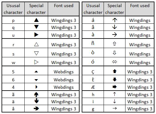
This uses specially chosen fonts to create the arrows. In the illustration below, the arrows are generated from the rendering of the characters  p, q w into the Wingdings 3 font:

The arrows are generated from a nested IF statement

=IF((D3-I3>0),"p",IF((D3-I3)<0,"q","w"))

with the resultant character 'translated' by formatting these particular cells to Wingdings 3. This method requires an additional column to create the panel. It has some advantages over the icon set method: It allows much stronger and sharper arrows which scale better; it allows much more flexibility in positioning; it allows the sizing of the arrows and percentage change figures to be treated independently; it opens up wider choice of symbols used.

Disadvantages are that the special font used needs to be installed on the reader's computer for the method to work (Wingdings 3 is part of the standard Windows build so is a fairly safe choice);  the method relies on character to symbol mappings which do not read intuitively in formulas . Also, this particular rendering of the method does not yet include tolerances, so additional work is needed to incorporate these.

Beyond symbols from the BBC example, there are many other options using this method. The following panel highlights a few:

Other approaches

Excel Shapes provide a number of potentially useful options. For example

These can be added and edited manually or controlled using VBA code. Manual editing makes updating tedious and prone to mistakes. VBA provides a fascinating intellectual challenge from a programming perspective (see References below) but then introduces further issues in how the spreadsheets are distributed and used. The variation in functionality through successive versions of Excel introduces further constraints i.e. it cannot be certain that what works on the originating computer will run or look the same for all end users.

Graphic image files, sourced from outside of Excel,  can theoretically allow for an infinite variety of shapes to be used, for example: 

The disadvantages of graphic image files are similar to those for Excel Shapes. 

Use of either Excel shapes or graphic image files would involve a much greater overhead in setting up and maintaining the spreadsheets compared with the font or icon set methods outlined above. This can only be justified if the desired graphic symbols really cannot be obtained any other way. Before embarking on a VBA heavy spreadsheet, it would be wise to consider honestly whether the desire to impress is eclipsing the desire to communicate. Similar pitfalls can occur with other visual choices in dashboard design.


Calculating what actually is up, down or the same

A change, say,  from 17,569 to 17,571 is, in strict mathematical terms, an increase of 2. The question, in dashboard design terms, is whether this should be considered as an increase or as no significant change. The answer to this will depend upon the specific context. This can then be expressed in calculations through assigning a "tolerance" value. The following panel illustrates how various value changes, all of which have exactly the same arithmetic difference, are interpreted at variety of different tolerances: 

Incorporating tolerances into dashboards

Tolerances can be added to dashboards and reports in a variety of ways. It cannot be assumed that one tolerance value will apply sensibly to an entire dashboard. In fact,  this is unlikely to be the case on many occasions. It is best to allow for each measure on the dashboard to have its own tolerance. 

In the next example, the font method described above has been adapted to include tolerances. An additional column is used to hold the tolerance values:  

The 'nested IF' formula from Method Two needs to be adapted in column E:

=IF((D3>(I3+(I3*H3))),"p",IF(D3<(I3-(I3*H3)),"q","w"))

Additionally, the conditional formatting of column F needs to be altered to keep it in step with column E:

Depending on how it is intended to be used, there is a further option to include the tolerances on the dashboard itself so the user can adjust the values.


References

Excel Dashboards & Reports (2nd Edition) by John Walkenbach and Michael Alexander. May 2013, Wiley.

Mastering Excel: Conditional Formatting by Mark Moore  Kindle Edition. May 2014 (link)

Icon Sets. Excel Easy
http://www.excel-easy.com/examples/icon-sets.html

Programming Excel 2007 and Excel 2010 AutoShapes with VBA by Nicholas Hebb. Peltier Tech Blog.  12th January 2010.

http://peltiertech.com/programming-excel-2007-2010-autoshapes-with-vba/

Working with shapes in VBA by Andy Brown. Wise Owl Training. 25 January 2014. http://www.wiseowl.co.uk/blog/s394/shapes.htm