Using a pie chart to show abundance over 12 months

When I'm not sitting at a computer trying to figure out how to get Excel to do things, I like to take wildlife photographs. I've just bought another old bird book from a charity shop: Jim Flegg's Field Guide to the Birds of Britain and Europe (New Holland. 1990)  Amongst other good things, it has an interesting type of chart in it (see the right hand side of the scan sample below):
















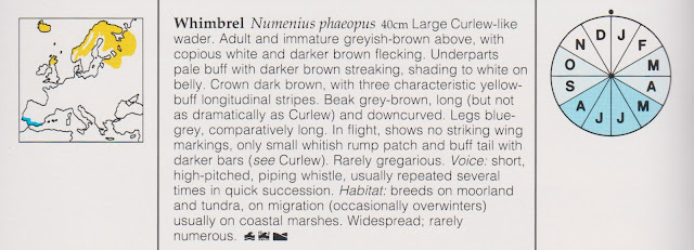
A simple three scale system is used to indicate, for each month of the year, whether the bird is 

• not likely to be seen  
• fairly likely or 
• highly likely

Although the chart looks superficially like a pie chart, it is more like a choropleth or heatmap. The slices are equal and never change size. They represent the twelve months of the year, running clockwise. The scale is a single-hue progression.


How easy is it to re-create this chart in Excel?

The challenge is to create a "dashboard" version of this chart such as

in which a bird can be selected from a drop-down list with the corresponding data automatically populating the chart.


Concentrating first on how to create the chart itself: It will obviously have to be rendered as an Excel pie chart. The particular issues to resolve are:

• How to display equal sized slices

• How to get the month identifier letters displayed inside the slices, rather than a number

• How to apply the differential slice tones 

The first two are relatively straight forward:

Giving each month an equal numerical value will make the slices the same size. For idiosyncratic personal reasons I have chosen to give each slice the value 30 (because 360 degrees cut into 12 slices would each be 30 degrees) but any equal number will work exactly the same in Excel.

To display the month letter (rather than the number 30) inside each slice, adjust the properties as follows

Use Format Data Labels:

• Set Label Options to 'Category name' (not to Value, the default)
• Set Label position to 'Inside end'

The 'tone' of the slices is set by the Fill properties. If you search the internet for ways to control this property you will generally end up programmatic solutions based on Visual Basic. This is an option.

But there is a way of achieving this without using Visual Basic. It requires setting up a Pie Chart with 36 slices.

Each month requires three slices. These are then manually formatted to provide the fills for 'None', 'Medium' and 'High'

The data settings for each month will then determine which slices are displayed:

In the illustration, the values for each month are set in column C

The values graphed are those calculated in column G. These will be 30 if the slice matches the value selected in Column C or otherwise will be zero.

The zero value slices will in effect be omitted. The formula controlling this in Column G is

=IF(H3=VLOOKUP(E3,$B$3:$C$14,2,FALSE),30,0)

The labels are based on column F, which take the first letter of the month name, or if there is a zero value slice are blank. This is calculated through the following formula in column F

=IF(G3>0,LEFT(E3,1),"")

That is all there is to it. To use it in a "real" dashboard, we would put the graph in a separate area (or sheet)  to the calculations and then link the selected values to a data table of all birds