Quads and Qwarters - an alternative to counting by months

Counting by months  is both deeply rooted and deeply flawed for many types of analysis and presentation. 

Months have varying duration and they start inconsistently on different days of the week. Any analysis of volumes by month introduces a layer of fog which can obscure the underlying patterns we are looking for.

Counting by weeks works much better. The periods are all the same length. And where the patterns of activity we are studying have an underlying shape based on days of the week, this is balanced out. A time series based on totals by week has the immediate advantage of comparing like for like.

But what do we do when we need a higher level view? Aside from the little problem of leap years, counting by years is a reasonably solid framework

In between, traditionally we would look at counting by months and by quarters. A better framework can be built up using multiples of weeks. 

So instead of 12 months of uneven length we can use 13 'quads' each of four weeks

And instead of 4 quarters of uneven length, based on months, we can use four identical length 'qwarters' each of 13 weeks

This gives balanced frameworks of comparable 'granularity' to their uneven traditional counterparts

The only big problem is deciding what to call them. Pending any better ideas, I have chosen to label the 4 week 'quads' 4w1 through to 4w13.

Similarly, I have used Qw1 through to Qw4 to match the familiar Q1 to Q4

Reference

E.Bolton. Why month-based views are unsuitable for data which exhibits weekly patterns. BI Dashboard Design. 02/02/2016

Bullet charts in Excel

This type of chart was devised by Stephen Few. His specification is at

https://www.perceptualedge.com/articles/misc/Bullet_Graph_Design_Spec.pdf

It is intended as a replacement for the ‘speedometer’ style dashboard gauges. These started appearing in the 1990s but are now regarded as a poor design choice.

The bullet chart shows a single measure. It can show this relative to several comparators. Typically this is a target and ranges of low, medium and high





For example, a bullet chart could be used to show NHS performance against the national target (95%) for 4 hour waits in A&E. This can be shown against a back-drop of the range of performance by peer organisations





Excel does not currently provide a bullet chart as part of its standard chart gallery. These charts can be produced in Excel. But doing this requires ‘bending’ Excel slightly to make it do what we need.

There are numerous blog articles available giving instructions on how to do this. I think Jon Peltier has produced one of the best. I have borrowed many of his ideas. Most solutions use a combination chart and adapted error bars.

There are some questions to answer before we start

• Do we want a horizontal bullet chart (bar) or a vertical (column)? 
• Do we want a single bullet chart on its own or several together? 
• Do we want a legend on the chart? 

I think the horizontal version works best (although it is slightly more complicated to set up in Excel). The sections below show how to do this in Excel.

Single horizontal bullet chart (with or without legend)

This method mixes three bar data series and two scattergram series (which we need to position parts of error bars from).

You will need to set out the source data as follows:




Step One

Highlight the cells which cover the Low, Middle and High ranges (yellow in the screenshot – do not highlight the entire block of data).

Use this range to insert a Clustered Bar Chart.

If the result looks like this





You will need to Select Data… and Switch Row and Column to get the following:




Step Two

If you want a legend, add it now.

Format the fill of the three bars to reflect the desired grey scale.






Then adjust the bar properties to 100% overlap and 50% gap width





Reduce the height of the overall chart to condense the bar height





Step Three
We now need to add the two remaining data series. We add them one at a time. Because we are using a scattergram type for these series, we need two measures for each point. The 'secondary y axis' measure is used to control the vertical position of the marker. 50% (or 0.5) will allow us to make it central

Select the Measure range and the Secondary Y axis range together (hold control key) then Copy






Click on the chart to select it.

Then select Paste Special and set options as follows





The new series should appear added like this





Select the new series and change its chart type to Scatter (X Y)




Step Four

If you want the legend, you will need to change the labelling and adjust the colour of the fill

If you do not want a legend, do not bother with this step as we will be hiding the marker later

Step Five



Adjust the secondary Y axis properties to run from 0 to 100% (this forces the 50% to the middle) then delete it

Step Six


Add the final data series in similar fashion to Step Three. Highlight the range (yellow in the screenshot) and Paste Special into the Chart

Step Seven

If you want the legend, reformat the data series and adjust the label

Step Eight

Add error bars to Target data series

Delete the horizontal error bars

Format the vertical error bars

• End style No cap
• Error amount fixed value 0.3
• Bar colour
• Increase Bar width to 1.5pt or greater

Then highlight the Target data point and set marker to None

This removes the marker leaving the error bar behind (and leaves the Legend intact if you want this)

Step Nine

Add error bars to Measure data series

Delete the vertical error bars

Format the horizontal error bars

• Direction minus
• End style No cap
• Error amount percentage 100%
• Bar colour as required (red in this illustration)
• Increase Bar width to 5pt or greater

Highlight the data point and set marker to None

Step Ten

Format to suit

If you don’t want the legend you can omit steps four and seven

Excel: creating a movable hairline date marker on a time series chart

If you want to add a marker line to a one-off chart it is probably easiest to use Excel's drawing tools (Shapes).

This article looks at a more complex situation. We want the position of the marker line to move automatically based on selections in the dashboard.

For example we may use a line chart to show a time series. A hairline marker could then be used to highlight a date of interest. The position of the marker should then move in line with currently selected values or changes to the data.

This can be set up in Excel relatively easily and without having to resort to any VBA code. The method shown here creates the hairline from a column data series aligned to a secondary axis. I devised this method myself - rather than borrowing it from any books or websites - so this may be the first time it has been described anywhere. Although given the ingenuity of Excel users,  I quite expect to find that others will also have invented it, or something like it

The illustration is a generalized chunk of a dashboard. The idea is that the user selects a week of interest using a drop down list. The data displayed is automatically updated to match the chosen week. The position of the hairline marker on the line chart also  moves to indicate the position of the chosen week, And the date displayed above the hairline is also updated to give the correct detail

I am not going to explain here how to update the table of values in line with the selected week. You will be able to do this in various ways including  using VLOOKUP() and/or INDEX()/MATCH(). The details will have to be tailored to your individual situation, in particular where you are getting your data from and how you plan to refresh it.

Neither am I going to explain how to create a line chart with a 'shadow band' effect covering a range of older data - I have covered this is an earlier article
http://bi-dashboard-design.blogspot.com/2018/05/the-problem-of-too-many-lines-on-time.html

The focus here will be on how to create the movable hairline. The main features are:

• The hairline is simply a standard Excel column data series with the properties set to make it very narrow
• The chosen week is displayed by being the only week that is not hidden.
• Hide all the other weeks by making their value calculate to #N/A when they are not chosen
• Use the secondary vertical axis to ensure that the height of the hairline remains the same whatever happens to the values in the line series
• Set the hailrlne data label by pointing it at a cell with the date in

None of this is difficult


Alternatives?

Another method from elsewhere is to use a scatterplot with an error bar

The problem of too many lines on a time series line chart

The challenge is how to show several years worth of data in a time series using lines. Even William Playfair struggled with this one















There are two approaches which might help us here

• Progressively fade the years out as they get further into the past
• Band several years together to produce a background range

This article shows how to do both of these using Excel.


The problem

We will use some data from my world - it  does not really matter what it is. We have weekly totals for five successive financial years

So we highlight the five years and insert Excel's default line chart, which produces this:

It's a horrible mess. Obviously we will work on it a bit: Move the legend to the bottom, stretch it out

It is still extremely hard to follow. The problem is that there are too many lines criss-crossing each other, and the colour of the lines has no real meaning

I regularly see charts like this  - often with even more lines. The analyst has simply trusted to Excel's standard chart gallery and colour schemes. Excel has blown them a raspberry. Excel is a brilliant software package, but you often have to twist its arm to get it to do what you need.

Progressively fade out earlier years

This approach tries to put meaning into the colour of the lines. Most of us will probably agree that it is worth looking at the position at the same point last year. Is the year before that of equal significance? Or the year before the year before? Probably not.  So this approach dilutes the visual impact of earlier years. You can still see them but they clash less.

This is a big improvement. We have used standard Excel colour palette options (we could use a  colour selecting utility to make ore precise custom choices). We have also adjusted the contrast of the gridlines, axis and legend labels,

While it is better, it is still very 'busy'. So the next step would be to sacrifice the oldest year of data

This is a lot clearer - it allows a greater contrast between the most recent year and the one before.

It's still quite busy. What does removing another old year look like?

That looks about right for this pattern of data.

We maybe need to double check that the our colour scheme is giving us something extra (rather than it just being  a result of reducing the number of data series),  So here is the same chart again using the the Excel default colours

Yes the 'fading' scheme is much clearer, and the other adjustments to contrast also help.

Band past years together

What if we do not want to lose sight of the earlier years? A way to retain some of this information is to calculate the range of vales for each week over several years. This takes a little bit more setting up.

First add some calculated columns for the Minimum, Maximum, Range (i..e Maximum - Minimum) and pull through the latest year as a repeat column

Then use the three columns Minimum, Range, Last Year to create the graph.

Start by inserting a Stacked Area graph

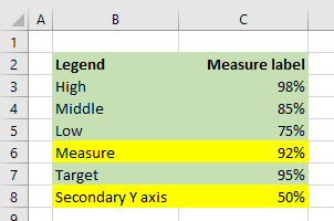
Next adjust the data series properties so that the Min series is invisible and the Range (Max-Min) is a faint colour

Next change the chart type for the Last Years (2017-18) data series from Stacked Area to Line

That's more or less it - it just needs some tidying up

• Move the legend  from the side to underneath
• Delete the Min from the legend
• Change the legend label for Min-Max to something more meaningful
• Adjust contrast on grid-lines and axis labels
• Adjust line colour of main series to taste

So that's about there now. It allows us to see what the weekly pattern of  the year in question was against the range of the four years before it 

For me this is the best way to look at this particular pattern of data. For other patterns I may think differently but it's a good starting point

The advantage of Excel is that you can quickly knock together different versions to see what they may show

Some other thoughts and possibilities

One approach that might be suggested from modern data visualization thinking is 'small multiples'. In this approach, rather than combining the years into a single chart, each year would be plotted singly and then all would be aligned into an overall view

Here's a quickly assembled version in 'small multiples' style

This is ok in the sense of showing the pattern for each year. But how easy is it to see whether 2017-18 values stray outside the 'typical' range?. Does this version of small multiples offer much more than simple sparklines?

So maybe to make caparisons easier in the 'small multiple' version we might have to add some solid fill?































Using a solid fill below the line, and containing the plot area makes the comparisons easier. But it still requires a lot of mental gymnastics to make and hold the comparisons

If you able to use these charts in an interactive setting then there are options for rotating through successive years using a pull-down list - as the following illustration roughly simulates:

Some Websites

Perceptual edge https://www.perceptualedge.com/ Probably the single best website for data visualisation. Stephen Few set up Perceptual Edge as a consulting company in 2003. This website contains a substantial collection of articles, available free. It also contains 20 examples of poorly designed charts and how to improve them. The blog provokes a lot of interesting debate. If you are only going to look at one website to learn about data visualisation, pick this one.

The Work of Edward Tufte and Graphics Press https://www.edwardtufte.com/tufte/ This is Edward Tufte’s website. I found it a little idiosyncratic at first. But if you persevere, it has some very stimulating and wide-ranging material. It provides a way to purchase Tufte’s books, including electronic versions of some works.

Peltier Tech Blog https://peltiertech.com/ This is Jon Peltier’s website. It contains a lot of practical ‘how to’ examples for getting Excel to do things. He ranges into all sort of Excel matters but there is a lot of good material on graphs and charts. He is particularly good at finding solutions for tricky problems. Evergreen Data http://stephanieevergreen.com/ This is Stephanie Evergreen’s website. She runs Evergreen Data and the website promotes this business. The Blog section contains a short selection of articles, some of which are reproduced in her books. It is quality rather than quantity. Recommended

ExcelUser http://www.exceluser.com/ This is Charley Kyd’s website. It is wide ranging and full of good tips. It includes quite a lot on Excel graphs and charts. Excel Charts https://excelcharts.com/ This is Jorge Camoes’s website. Although it is entitled ‘excel charts’ it ranges much wider than being a simple excel ‘how-to’ site. There is a lot of discussion about what makes good visualisation.

Chandoo.org https://chandoo.org/ Chandoo is one of the Excel lifelines that I have dipped into over the years. He covers charts (and dashboards) extensively. Sometimes the graphic style drifts away from my liking – but that is a matter of personal taste not technique.

Color Brewer 2.0

http://colorbrewer2.org/#type=sequential&scheme=BuGn&n=3 If you need to set up a visual hierarchy using colour, this site takes away a lot of the hard work. It allows various numbers of levels to be applied to different colour sets. It gives the technical specification of the colours which can then be used to transfer to your software.

A set of data presentation standards from 1915

If you are interested in data visualisation you may think that modern data visualisation thinking started with Edward Tufte in the 1980s. You may follow the trail back to John Tukey in the 1970s or even to Mary Eleanor Spear in the 1950s.

In fact we can track back over 100 years. Williard Brinton's landmark book Graphic methods for presenting facts was published in 1914.  The Joint Committee on Standards for Graphic Presentation,  propelled by Brinton,   published its first (draft) set of standards in 1915. These  are surprisingly relevant even now:



Standard 1

Standard 2

Standard 3

Standard 4

Standard 5

Standard 6

Standard 7

Standard 8

Standard 9

Standard 10

Standard 11

Standard 12

Standard 13

Standard 14

Standard 15

Standard 16

Standard 17